The kind of source files we have in mind are sequences of characters
(for example, text files), sequences of bits (for example, binary code
of a computer program), or sequences of numbers (as occur in digitized
audio and image files). Let us distinguish between two kinds of compression:
When we are working with text files or with binaries, we want to be able
to recover S exactly upon decompression, while for audio and image files
we only need to be able to recover something that sounds or looks as good
as the original. The former kind is called "lossless" compression,
since we do not lose any information when we compress, while the latter
is called "lossy" compression. We'll begin with lossless compression.
2 1 + 22 + ... 2n-1 = 2n -2 < 2n.
This means that any algorithm that compresses every file of length n must produce the same output file on two different inputs; thus we could not reliably recover the source file from the compressed version. Put another way, if we can always recover the source file from the output of an algorithm, then the algorithm cannot compress everything---some files will actually get larger when you apply the algorithm.
Exercise. No free lunch with WinZip
(a) If our source file consists of a million bits of the sequence
1010101010101010101010.....
we can just send a five-line C program that writes the bit sequence 10 five hundred thousand times, instead of the source file.
(b) Suppose our source file is the bitmap of a line drawing. Black pixels in the drawing itself are represented by 1, white pixels in the canvas are represented by 0. Now typically such a bit map will contain many more zeros than ones. For example, on a screen 1000 X 1000 pixels, we might have on the average four black pixels per row, or about 4000 ones altogether. We can thus transmit, instead of the source file, the number of zeros between successive ones. This requires transmission of about 4000 32-bit integers---thus 128,000 bits instead of 1,000,000.
(c) Here is a variant on the preceding example. Imagine a message consisting of the letters A, B, C and D. We could code each of these letters by a pair of bits, for example 00 for A, 01 for B, 10 for C, and 11 for D. Suppose, however, that A occurs more frequently than the other letters. For instance, suppose 80% of the letters are A, 10 % are B, 7% are C and 3% are D. We could then encode A by 1, B by 00, C by 010 and D by 011. Observe that with this scheme there is only one way to decode a string of A's, B's, C's and D's, and that the average number of bits per symbol is
0.8 x 1 + 0.1 x 2 + 0.07 x 3 + 0.03 x 3 = 1.3,
which is considerably less than the two bits per symbol of the orignial coding scheme.
(d) Suppose, in contrast, that our message is a completely random sequence
of A's, B's, C's and D's (whatever that might mean). The coding scheme
used in (c) would actually require more than two bits per symbol.
Now imagine an unknown passage of English text. Suppose we are
told that the fifteenth character is a Q, and
suppose we know, for the sake of argument, that the letter Q occurs
in text on the average about once every two hundred characters. We
have thus reduced the search space by a factor of 200. This is equivalent
to halving the size of the search space between 7 and 8 times. We
thus say that we have provided log2200=7.6 bits of information.
In general we say that a symbol that occurs with a probability of p carries
log2(1/p) bits of information.
Now suppose that a message is drawn from a set of messages over an alphabet of symbols {b1,..,bk}, and suppose that the symbol bi occurs with a relative frequency of pi. In a typical message of length n, each symbol bi will occur about npi times, and thus the total amount of information in the message is, on the average
np1log2(1/p1)+...+npklog2(1/pk)
bits. The average amount of information per symbol is thus
p1log2(1/p1)+...+pklog2(1/pk)
bits per symbol. We call this quantity the average entropy of the set of messages, or, by a slight abuse of terminology, the average entropy of the message itself.
log23 = 1.58
bits per symbol. In general, if the underlying alphabet has n symbols, which occur with equal frequency in the message, then the entropy is log2n bits per symbol. This represents the maximum attainable information content. (The intuition is that a truly random message, which would exhibit such a uniform distribution of symbols, cannot be communicated with a smaller number of symbols.)
2. At the other extreme, a message consisting entirely of 1's or of 0's has entropy 0. A message that consists of 99% 0's and 1% 1's has entropy
0.99log2(1/0.99)+0.01log2(1/0.1) = 0.081
bits per symbol. This suggests that in such a message one million bits long, there are only eight thousand bits of information.
Exercise : Compute the entropy of Bleak House
3. The standard ASCII code represents a character by a one byte (= 8 bits). However, the leading bit of this byte is always 0. Thus a long text file can be viewed as a string of bits in which every eighth symbol is 0. Let's assume (although for ordinary text files this is surely not true) that 1's and 0's occur with equal frequency in the remaining seven-eighths of the bit positions. The probability of occurrence of a 1 is thus 7/16, and of a 0 is 9/16. The average entropy is consequently
(7log2(16/7)+9log2(16/9))/16=0.9888
bits per symbol.
Exercise : A simple text-compression scheme
0101010101010101.......
The average entropy is one bit per symbol, because 0's and 1's occur with equal frequency. But surely that is not the whole story, since intuition strongly suggests that this sequence carries very little information. In fact, if we grouped the symbols in pairs
01 01 01 01 ...
and regarded each pair as a single symbol, then the entropy would be 0. Thus the first-order entropy, which is what we were looking at in the last section, overestimates the information content of the message. Sometimes we will be interested in higher order entropy, which we obtain by looking at pairs, triples, etc., of symbols, and considering each such block as a single symbol.
Example: Suppose we have a long sequence of alternating
0's and 1's, as above, sporadically interrupted by an
extra 0 or 1, for example
1010101010101101010101010101010100101010101010101
When we break this into blocks of two symbols we get
10 10 10 10 10 10 11 01 01 01 01 01 01 01 01 00 10 10 10 10....
Let us suppose that the interruptions are rare enough that 49% of the pairs are 10, 49% are 01, 1% are 00, and 1% are 11. If we consider each such pair as a single symbol, the entropy is 1.14 bits per symbol, or 0.57 bits per bit of the original message.
Exercise : Compute the second-order entropy of Bleak House
Exercise : Synthetic
English
Example. This reprises an earler example. Suppose we are encoding messages over the alphabet {a,b,c,d}. A natural scheme would be to encode the four letters by the bit sequences 00, 01, 10, and 11, respectively. In this case, a message of length n would be encoded by a bit string of length 2n, an average of two bits per symbol. Suppose, however, that the nature of the messages was such that the symbol a occurred five times as often as each of the other symbols---that is, a occurred with a probability of 5/8, and each of the other three symbols with a probability of 1/8. We might then choose to encode a by 0, b by 10, c by 110 and d by 111. The average number of bits per symbol would then be
5/8 x 1 + 1/8 x 2 + 1/8 x 3 + 1/8 x 3 = 1.625
For such a scheme to work, we need to be able to recover the source message from the encoded message, so there must be only one way to decipher an encoded message. A little experimenting should convince you that the encoding scheme in the example above satisfies this property. (In this connection, see the section on prefix codes below.) Had we chosen, however, to encode a by 0, b by 01, and c by 10, we would have a problem, since 010 can be decoded as either ac or ba. Thus we are only interested in uniquely decipherable codes.
Here is a fundamental theorem of information theory. Suppose we
have an alphabet of k symbols{b1,...,bk}, and that
bi is encoded by a string of ni bits. Suppose
further that this code has the unique decipherability property. Then
![]()
From this it is not difficult to deduce that if a message of length N over the alphabet {b1,...,bk} has entropy H, then the number of bits in the encoding of this message is at least HxN, so that the average number of bits per encoded symbol is at least H.
This theorem gives a limitation on how far we can compress a message. To put it more simply, if the information content of a message is m bits, then we need at least m bits to encode it.
Exercise 5. Some theoretical questions for the mathematically minded.
Example. In our previous example with the alphabet {a,b,c,d}, the entropy is
5/8 x log2(8/5) + 3 x 1/8 x log28 =1.5423,
which is less than the average number of bits per symol in the coding scheme described above. This is what the fundamental theorem predicts.
Example. We've seen that we can encode a single 8-bit ASCII
character by a 7-bit string simply by lopping off the leading 0.
This is a uniquely decipherable code that uses 0.875 bits to transmit each
bit of the source message. Compare this with the entropy of 0.973
that we calculated earlier for a bit sequence in which every eighth bit
ix 0. We appear to have violated the fundamental theorem! Or
have we? In fact, the set of symbols that we are encoding is the
set of eight-bit ASCII codes, not the individual bits. A truly random
sequence of such symbols has entropy of 7 bits per symbol, which is exactly
what our encoding gives; ordinary text would have even smaller entropy,
so this is entirely consistent with the fundamental theorem.
Example. {0,10,1110} is a prefix code.
Example. {0,0010} is a uniquely decipherable code, but it's neither a prefix code nor a suffix code (i.e., the reversal of a prefix code). This example shows that there are other ways to get uniquely decipherable codes.
Let us take a binary tree and label the nodes by bit strings, so that
the root is labeled by the empty string, branching left means 'append a
0', and branching right means 'append a 1'. Then the leaves of the
tree form a prefix code, because no leaf label can be an initial segment
of the label of another leaf.
Conversely, every prefix code can be represented by a tree in this fashion.
1. Initially, the collection consists of k trees, each with a single
node, bearing the labels p1,...,pk
2. Among the root nodes of the collection of trees, pick the two n1
and n2 with the smallest labels x1 and x2.
3. Create a new node with label x1+x2 and make
n1 and n2 its children. The collection now
contains one less tree than before.
4. If there is more than one tree in the collection, go back to step
2.
The resulting binary tree can then be interpreted as a prefix code; the bit string associated with the leaf labeled pi is the encoding of bi.
Example. Suppose the message consists of the letters A,B,C,D,E
and that these occur with relative frequencies 0.2,0.1,0.25,0.15 and
0.3 respectively. The figures below show the successive steps
in the construction of the Huffman prefix code for this message

The resulting prefix code is A-00, B-100, C-01, D-101, E-11. The
average number of bits per symbol in the encoded
message is then 2 x 0.2 + 3 x 0.1 + 2 x 0.25 + 3 x 0.15 + 2 x 0.3 =
2.65 bits per symbol. In contrast, the entropy is 2.228 bits per
symbol, while if we used a fixed-length encoding, we would be obliged to
use 3 bits per symbol.
If the entropy of the message is H then the average number of bits per character in the Huffman-encoded message does not exceed 1+H. Moreover, it can be shown that among all prefix codes, the Huffman code yields the smallest average number of bits per character.
Exercises
6,7. A series of problems on Huffman Coding
Here we describe the Lempel-Ziv algorithm called LZW. (The "W" stands for Welch, who published this particular variant of one of the original Lempel-Ziv algorithms.)
1. Initially, set Dictionary to be the set of input symbols (typically, these will be the byte values 0..255). Set prefix to be the empty string, and nextchar to be the first symbol in the message.
2.While prefix + nextchar (i.e., the string formed by concatenating nextchar to prefix) is in the Dictionary, set prefix to prefix + nextchar and nextchar to the next symbol in the message.
3. Output the position of prefix in the dictionary and add prefix + nextchar to the dictionary. If nextchar is the end-of-file marker, stop. Otherwise, set prefix to be the empty string, and go back to step 2.
Let's illustrate the operation of this algorithm with the symbol alphabet {a,b,c} and the message abababbc.
Step 1. Initially, the dictionary is (a,b,c) and the positions of these symbols are 0,1,2.
Step 2. a is in the dictionary but ab is not.
Step 3. Output 0 (the position of a), and add ab to the dictionary
Step 2. b is in the dictionary, but ba is not.
Step 3. Output 1, the position of b, and add ba to the dictionary.
Step 2. a and ab are in the dictionary, but aba is not.
Step 3. Output 3, the position of ab, and add aba to the dictionary.
Step 2. a and ab are in the dictionary, but abb is not.
Step 3. Output 3, the position of ab, and add abb to the dictionary.
Step 2. b is in the dictionary, but bc is not.
Step 3. Output 1, the position of b, and add bc to the dictionary.
Step 2. c is in the dictionary, but c + end-of-file marker is not.
Step 3. Output 2, the position of c in the dictionary and stop.
The output is 0,1,3,3,1,2. How does this compress the file? Each of these symbols can be encoded with two bits, so we wind up transmitting 12 bits, instead of the 16 bits we would require if we had encoded each symbol in the alphabet by two bits. That's not very impressive---even less so when you consider the fact that if the original symbol alphabet had been {a,b} and the message abababbb, then we would still wind up 12 bits when the original message could have been sent with 8 bits! The real power of the method does not become evident until we work with longer messages, when we would start to see many repetitions of short strings like ab, ba, abb, and wind up adding longer and longer strings as dictionary entries.
How does decompression work? We don't need to transmit any additional information with the message; the decoder will construct the dictionary in the same order the encoder constructed it.
For example, with the message above, 0 will be decoded as a, then 1 as b and ab will be added to the dictionary at postion 3. Then 3 will be decoded as ab and ba will be added to the dictionary. The next 3 will be decoded as ab, and aba will be added to the dictionary. Then 1 will be decoded as b and abb will be added to the dictionary. Finally 2 will be decoded as c, and bc will be added to the dictionary. The output is thus the original message abababbc.
Decoding is not always quite as straightforward as that. Let's consider what happens when we encode the message aaaaaa:
Step 1. Initially, the Dictionary is {a}.
Step 2. a is in the dictionary, but aa is not.
Step 3. Output 0 (the position of a) and add aa to the dictionary.
Step 2. a and aa are in the dictionary, but aaa is not.
Step 3. Output 1 (the position of aa in the dictionary) and add aaa to the dictionary.
Step 2. a, aa, and aaa are in the dictionary, but aaa+end-of-file marker is not.
Step 3. Output 2 (the position of aaa in the dictionary) and stop.
The output is 0,1,2. The decoder, on seeing this, decodes 0 as a, but then sees the symbol 1 before it has had a chance to add item 1 to the dictionary. We can get around the problem by analyzing how this situation can arise. Suppose the encoder output is a sequence of positions p0,p1,p2,..., and suppose further that pi is encountered by the decoder before the decoder has had a chance to add it to the dictionary. i cannot be 0, because p0 must encode an individual alphabet symbol, and these are put in the dictionary at the outset. It must be the case (you have to think hard about this!) that the string in position pi is obtained by concatenating the string in position pi-1 with the first symbol of the string in position pi-1. This observation enables us both to decode pi and to add the appropriate string to the dictionary.
Here then, is the description of the decoding algorithm. The encoded file is a sequence of integers. If index is an integer, then dictionary[index] denotes the dictionary entry at index, and first(dictionary[index]) denotes the first symbol of that entry.
put the alphabet symbols in the dictionary
read index from encoded file
prefix = dictionary[index]
output dictionary[index]
while there are still items in the encoded file
{
read index from the encoded file
if there is a dictionary entry for index
{
output dictionary[index]
put prefix + first(dictionary[index])
in dictionary
prefix = dictionary[index]
}
else
{
output prefix + first(prefix)
put prefix + first(prefix)
in dictionary
prefix = prefix +
first(prefix)
}
}
Let's see how this decoding algorithm works with the encoding of aaaaaa
in the example above. Initially, the symbol a is placed in
the dictionary. 0 is read from the encoded file, a is output, and
prefix is set to a.
We then read 1 from the encoded file. Since there is no dictionary
entry for 1, we output a+a=aa, put aa in the dictionary, and then set prefix
to aa. We then read 2 from the file. Since there is no dictionary
entry for 2, we output aa+a=aaa, set prefix to aaa, and put aaa in the
dictionary. Since no input remains, the algorithm terminates, with
output aaaaaa.
Exercise
8. A series of problems on LZW.
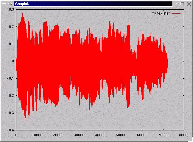
Shown below are two plots of sampled data from a recording of a flute. The samples were taken at interval of 1/11025 sec. The first plot shows about 6 sec. or so of samples, the second about 1/20 sec.taken from somewhere near the start of the recorded passage. Even in the close-up view, he sample points are close enough together to give the impression of a smooth curve when they are connected by line segments. By the way, the very sinusoidal appearance is not at all typical of recorded sound---it matters that this is a piece of recorded music played by a single instrument, and that the instrument is a flute. (Incidentally, the numbers on the y-axis are artifacts of the way the plot was made and have no particular significance---the actual values from the file were all in the range from 0 to 255.. The x-axis enumerates the samples.)

If the sampling rate, that is, the frequency with which measurements are made, is too low, the quality of the reproduced sound will suffer in two different ways. First, obviously, high-frequency components of the sound will not be accurately reproduced. Second, and less obviously, high-frequency components of the sound will be inaccurately reproduced, and show up as spurious low-frequency noise. This phenomenon, known as aliasing, is seen very vividly in movies, where the wheels on a speeding car will appear to be turning very slowly, or even slowly backwards. The reason is that the number of frames per second is much smaller than the number of revolutions of the car's wheels per second, so the camera catches the wheel at a sequence of positions that the eye assembles into a slow continuous rotation.
These effects are largely eliminated in high-quality digitized audio by first filtering out any component of the original signal above about 22kHz, since the human ear does not respond to frequencies higher than this, and then sampling at at least twice this rate. Thus CD-quality audio is created by sampling at a standard rate of 44100 samples per second.
A second source of distortion can occur when we store the measured amplitude as a number. If we were to allocate, say, four bits for this, then we are allowing for only 16 different amplitude levels over the whole dynamic range of the signal. The resulting distortion is called quantization error. A safer bet is to allocate 8 or 16 bits per sample.
So a three-minute song on a CD consists of two channels, each with 44100
x 180= 8 x 10⁶ measured samples, each of which takes up two
bytes; that is, about 16 megabytes in all. Sound files are huge.
Exercise
9. Some simple experiments with the .WAV file format.
Exercise 10. Some simple experiments with the .PPM file
format.
![]()
Let us give first the physical interpretation of these numbers. In our applications, the numbers (c0,...,ck-1) will be a sequence of sampled audio data (and, in particular, real numbers). These data are thus considered a discrete approximation to a continuous signal 1 time unit in duration. The discrete Fourier transform approximates the coefficients in the Fourier series of this continuous signal, which expresses the signal as a linear combination of sinusoidal functions
![]()
Since the original signal is real-valued, there is a symmetry in the transform values:
![]()
for i=1,...,k-1 (where the bar over a complex number denotes its complex conjugate).
The modulus |dj| of dj, for j=1,...,k/2, is then approximately the magnitude of the Fourier coefficient of the sinusoid whose frequency is j cycles per unit time; you can think of it as the strength of the signal at this frequency.
Let's see what all this means in terms of the flute data plotted above. I chose a sequence of 8192 consecutive samples from this signal and computed the Fourier transform [d0,..,d8191]. The moduli of these transform values were then plotted in the "wrapped-around" order [d4096,d4097,...,d8192,d0,d1,...,d4095,d4096]. The plot then displays the symmetry noted above.
![]()
The sharp spike at 0 is the "DC-component" of the signal. This is the modulus of sum of the original sample values. Changing the DC component without altering the other transform values has no effect on the sound of the original signal, but is rather an artifact of the range that was chosen to represent the sampled amplitudes. There is a very large spike corresponding to a frequency of about 500 cycles per unit time. Since the unit of time here is 8192/11025 = 0.74 sec., this represents a frequency of about 500/0.74 = 676 hz. (To locate this musically, C above middle C is about 500 hz., and the next higher C is about 1000 hz,. so this is somewhere between the two.) The other two spikes appear to be at integer multiples of this frequency. I suspect that the chosen passage consisted of a single note, and that these two spikes are the natural harmonics of the fundamental frequency.
Most of the remaining transform values appear to have moduli very close to 0. (A closer inspection of the transform values shows that they are not quite zero, but in any case they are very small compared to the spikes.) If they really were 0, then the sequence of transform values would consist mostly of zeros, and consequently have very low entropy. We can make a first stab at a lossy sound compression algorithm based on this idea:
1. Compute the DFT (d0,...,dk-1) of the
sampled data.
2. Quantize the values d1,d2,...,dk/2:
This is a sequence of k/2 complex numbers. One way to perform the
quantization is to let rmin and rmax denote
the minimum and maximum real parts of these number, imin and
imax the minimum and maximum of the complex numbers, and then
divide the intervals [rmin,rmax] and [imin,imax]
each into 256 subintervals. This enables us to encode each complex
number by two bytes.
3. Apply some lossless compression technique, such as Huffman coding,
to the resulting sequence of k bytes.
4. Transmit the 5 floating-point values d0,rmin,rmax,imin,imax,
followed by the Huffman coding of the k bytes.
With any luck, we should see very small values(like 0,1 and 2) predominating among the k bytes, and thus fairly low entropy.
To decompress, we first use Huffman decompression to restore the k bytes
used to encode the tranform values, then use the five real numbers
and the conjugate symmetry to reconstitute the transform. Note that
there will be some quantization error. Finally, we apply the inverse
Fourier transform to reconstitute the original signal.
Exercise 11. Try out this compression algorithm out.
Let's recall some mathematical and algorithmic properties of the DFT. The DFT is a linear transformation on complex k-dimensional space. This means that the DFT represents a change of basis of complex k-dimensional space: If (c0,...,ck-1) is a vector, then its transform represents the coordinates of the same vector with respect to the new basis.
Moreover, it's a unitary transformation, which means that the transformed basis is essentially a rotation of the original standard basis. (Well, not quite---it would become a unitary transformation if we divided each component of the transform by the square root of k. This introduces a scaling factor into our subsequent computations, but doesn't affect the general validity of what we're saying.) This has several practical consequences. First (by the very definition of unitary transform), the inverse transform is the conjugate transpose of the transform, which means that the formula for the inverse transform is just about the same as that for the transform itself;
![]()
Secondly, if (d0,...,dk-1) is the
transform of (c0,...,ck-1), then (up to the scaling
factor) the norms of these two vectors are equal:
![]()
Thus the contribution of a component to the overall strength of a signal is the same whether we are looking at the time domain (the original samples) or the frequency domain ( the transformed values). This leads one to believe that if we replaced the smallest components of the transform by 0 before applying the above algorithm, we might achieve even further compression, without appreciable loss of signal quality.
Exercise 12. Try this compression idea out.
Finally, the DFT can be computed very efficiently. Although a direct calculation of the DFT of a k-dimensional vector would require about k2 complex multiplications and k2 complex additions, the Fast Fourier transform algorithm reduces the number of complex arithmetic operations to a small multiple of k log k.
Here are the results of some experiments using the above compression
techniques. I computed the Fourier transform of the first 216
entries in the file flute.wav, then set to 0 all transform values whose
modulus was below a certain threshold, then quantized, replacing each complex
transform value by a pair of bytes. Because of symmetry, only half
the transform values need to be saved. The result
was then inverse transformed, and repacked back into a .wav file, to
hear the effect on the sound, and also compressed, using a lossless compression
method (UNIX compress).
Listen to the result when 87% of the transform values are set to 0. The byte values representing the transform can be compressed, using UNIX compress, to a file of 7877 bytes, or 12% of the original file size.
Listen to the result when 95% of the transform
values are set to 0. The byte values representing the transform
compress to a file of 4367 bytes, or 6.7% of the original file size.
![]()
The original array can be recovered by applying the inverse transform:
![]()
(Note added later---there is an error in the above formula: There should be a minus sign on the second exponent as well as the first.)
How can we compute the two-dimensional transform efficiently? Two facts are useful here: We can compute the 2D transform by first computing the DFT of each row, giving a new array, and then computing the DFT of each column of the resulting array. Thus if we use a fast transform algorithm, the total number of complex arithmetic operations performed will be a small multiple of N2log N, instead of the N4 we would get by straightforward implementation. Secondly, if we begin with real data, which will be the case for image files, then we only need to compute half the transform values; the other half can be inferred from symmetry in the data.
Exercise 13. Justify these claims.
Intuitively, "high frequency" in an image corresponds to very small-scale detail, and low frequency to large monochromatic regions. Because of the norm-preserving property of the DFT, we ought to expect that when we kill off small components in the transform and then apply an inverse transform, the result ought to be close to the original.
Exercise 14. Repeat exercises 11 and 12 for our image files.
How well does this work? On the one hand, you can always recover the original data values from the transform values, so in principle it should still be the case that eliminating small transform values should not change the image too much. However the transform of an image file is unlikely to consist of just a few sharp spikes with a large number of very small values. If you traverse one row of a digitized photograph, you will probably see a few sharp transitions between light and dark, and the transforms of such sequences tend to have non-negligible values across a large range of frequencies.
Quantization also presents something of a problem. When I tried
out the 8-bit quantization algorithm described above and then applied the
inverse transform, without eliminating any transform values, the image
quality was significantly degraded. I found it necessary to use 16-bit
quantization, so that the file encoding the transform, prior to lossless
compression, is twice as large as the original image file.
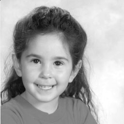
Having said all that, it's remarkable that this method of image compression works as well as it does, though it works much less well than Fourier compression of sounds. Here is our original test image:
Here is the result of transforming, killing all but 25% of the transform values, quantizing with 16-bit quantization, then transforming back. The resulting byte encoding of the transform, when compressed, takes up 34KB, or a little more than half the original file size.

And here is the result of transforming, killing off all but 9% of the
original tranform values, and transforming back. The compressed file
is 14.6Kbytes, about 22% of the original size.

The black splotches on the right show up, I believe, because a value
that was originally 255 (all white) in the original image, after transforming,
quantizing, and inverse transforming, turned into 256, which got written
as 0. A little more care in writing the program would have fixed this!
Consider the following sequence of 8 vectors. Each vector consists of 1's, -1's and 0's, and is multiplied by a scalar:
v0 = 2-3/2(1,1,1,1,1,1,1,1)
v1 = 2-3/2(1,1,1,1,-1,-1,-1,-1)
v2 = 2-1(1,1,-1,-1,0,0,0,0)
v3 = 2-1(0,0,0,0,1,1,-1,-1)
v4= 2-1/2(1,-1,0,0,0,0,0,0))
v5= 2-1/2(0,0,1,-1,0,0,0,0)
v6 = 2-1/2(0,0,0,0,1,-1,0,0)
v7 = 2-1/2(0,0,0,0,0,0,1,-1)
The dot product <vi,vj> of any two distinct vectors in this list is 0, which means that the 8 vectors are mutually perpendicular. The scalars were chosen so that the length of each vi is 1. Thus this collection of vectors forms an orthogonal basis for real 8-dimensional space. An analogous set of n n-dimensional vectors with the same properties can be constructed whenever n is a power of 2. We'll stick with 8 for our elementary examples, and use 256 for our image compression experiments.
The Haar wavelet transformation of a real vector c = (c0,...,c7) is the vector d = (d0,...,d7), such that
c = d0v0 + ...+ d7v7.
A basic property of orthogonal bases implies that
di = <c,vi>
For example, if c = (1,2,3,4,4,3,2,1), then
d0 = 20/23/2
d1 = 0
d2 =-2
d3 = 2
d4 = d5 = - 2-1/2
d6 = d7 = 2-1/2
Thus we can compute the Haar wavelet transform of an n-dimensional vector by forming n dot products, which means n2 multiplications.
There is a faster algorithm for computing the transform. Let us start with an n-dimensional vector c, where c = 2k for some positive integer k.
Step 1. Replace (c0,c1) by ((c0+c1)/21/2,(c0-c1)/21/2). Likewise replace (c2,c3), (c4,c5), etc.
Step 2. Repeat Step 1, but apply it only to the subvector consisting of components 0,2,4,.... Components 1,3,5,....are unchanged.
Step 3. Repeat Step 3, but apply it only to the subvector consisting
of components 0,4,8,...
.
.
Step k. Repeat Step 1 on the subvector consisting of components
0 and k/2.
Let's see how this works on our vector (1,2,3,4,4,3,2,1). We'll eliminate the divisions by the square root of 2 until the end:
The first step gives (1+2,1-2,3+4,3-4,4+3,4-3,2+1,2-1)=(3,-1,7,-1,7,1,3,1).
The second step gives (3+7,-1,3-7,-1,7+3,1,7-3,1)=(10,-1,-4,-1,10,1,4,1).
The third step gives (20,-1,-4,-1,0,1,4,1).
Now let's restore the divisions: Components 0 and 4 get divided three times by the square root of 2, components 2 and 6 twice, and components 1,3,5, and 7 once. So the result is
(20/23/2,-2-1/2,-2,-2-1/2,0,2-1/2,2.2-1/2)=(d0,d4,d2,d5,d1,d6,d3,d7), which are the transform components in permuted order.
To compute the inverse transform we simply reverse the steps above, applying the basic move first to components 0 and k/2, then to components 0,k/4,k/2, and 3k/4, etc.
The number of additions and multiplications is proportional to n.
What's the point of all this? Consider a vector like (0,0,0,...,0,1,1,1,1,0,0,.....0). If you think of these as gray-scale values in one row of a digitized photograph, the vector represents a constant color for part of the row, a sudden jump from dark to light, and then a jump back to dark for the rest of the row. Such transient phenomena are common in images. The Fourier transform of such a vector will tend to exhibit components of non-negligible size across a wide range of frequencies, which makes compression difficult. But the wavelet transform is sensitive to both differences in frequency (small-scale versus large-scale variation) and differences in locale (where a small-scale variation occurred). The Haar wavelet transform of this vector will have many components equal to 0 and many quite small.
Exercise 15. Some basic exercises with the Haar wavelet transform.
The idea is the same as before: We compute a two-dimensional
Haar wavelet transform of a digitized image by transforming each row, and
then transforming each column of the result. We set small components
of the transform to 0, and quantize. The quantized transform, we
hope, has low entropy and can compress well using lossless techniques.
The inverse transform applied to the quanitized transform is we, hope,
a good reproduction of the original image. Here are some results.
As before, 8-bit quantization produces crummy results, even if we don't
throw away any transform values. I used 16-bit quantization for the
experiment below. The image was created by killing all but 9% of
the Haar wavelet components of the image transform. The resulting
byte file compressed to 15KB, which is 23% of the original size.
I fixed the problem of the black blotches.
