CS345, Machine Learning
Prof. Alvarez
Probability Density Estimation using Kernels
Many machine learning techniques require information about the probabilities
of various events involving the data. A Bayesian approach, for instance,
presupposes knowledge of the prior probabilities and the class-conditional
probability densities of the attributes. This information is rarely
available and must usually be estimated from available data.
Here I illustrate one approach to estimating probability densities
using kernel functions.
Kernel Functions
In the present context, a kernel function is simply a predefined
probability density, usually something simple like a Gaussian or a bump
function. I will assume that the data are 1-dimensional, so that a kernel
is a function of a single variable x.
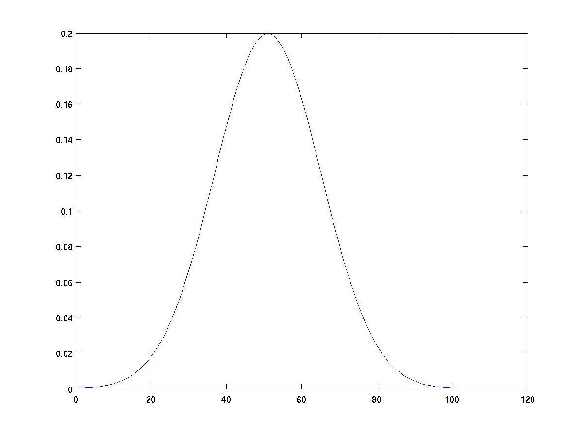
Here is an example of a Gaussian kernel. Note that the values on the
horizontal axis are given as multiples of 0.1, for example the points
labeled 80 and 100 are actually (100-80)*0.1 = 2 units apart.
The area under this curve is really 1 as it should be.

Scaled kernels
Formally, a kernel is a function K(x) that satisfies the following properties:
- K(x) ≥ 0 at all points x.
- The area under the graph of K(x) equals 1.
A kernel function may be scaled by selecting a width parameter w
and considering the new function (1/w)*K(x/w). This new function
is also a kernel (check that this is true).
Kernel-Based Estimation
The kernel-based approach to density estimation is very simple.
A kernel is first selected in advance, together with the desired
kernel width. The density estimate (function) is initialized to 0 everywhere.
One then makes a scan over the set of training instances. Each
instance contributes to the total density estimate by adding
one copy of the scaled kernel centered at the instance in question.
The sum is normalized by dividing by the number of instances.
Kernel Estimation Pseudocode
	Inputs: kernel function K(x), kernel width w,
		training data instances x1...xn.

	Outputs: an estimate of the probability density function
		underlying the training data.

	Process:

		initialize dens(x) = 0 at all points x

		for i = 1 to n:
			for all x:
				dens(x) += (1/n)*(1/w)*K((x-xi)/w)
Example
I performed density estimation on 100 data instances generated using
a mixture model. The data are available here.
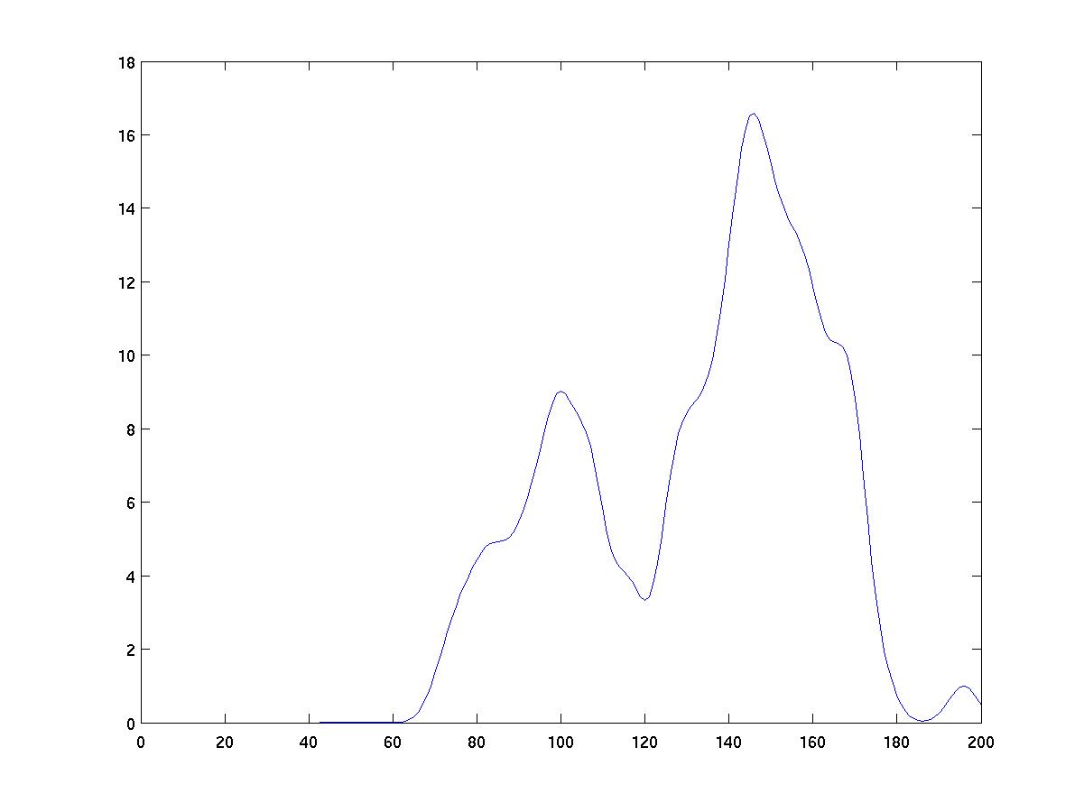
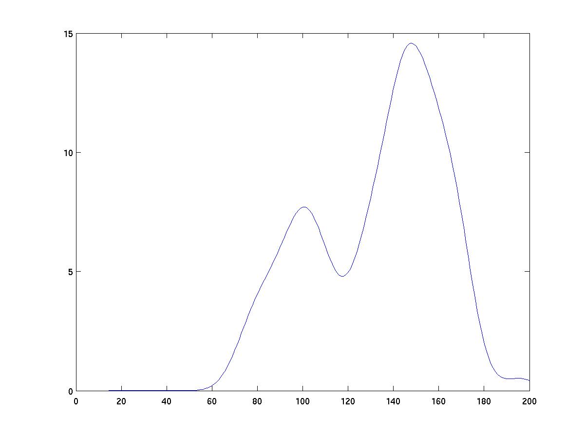
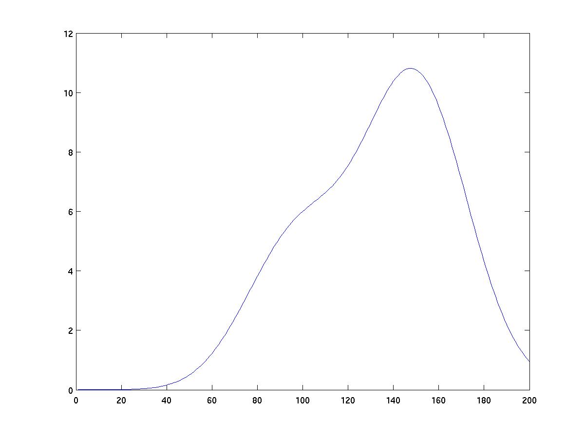
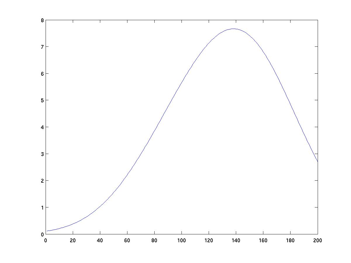
The kernel used for estimation was Gaussian. The results for
different kernel widths appear below.
Discussion
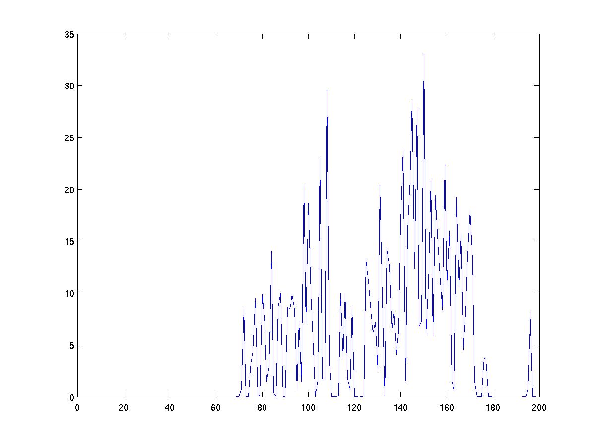
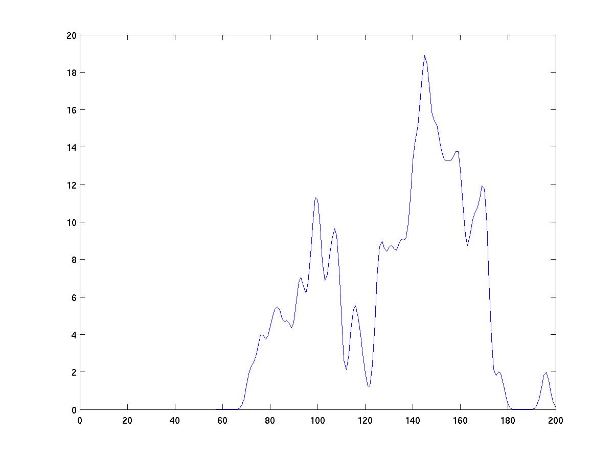
As you can see from the figures below, the choice of kernel width
has a big impact on the results of density estimation. Too narrow
a kernel yields "spikes" near individual data instances. Too wide
a kernel smears out all detail. The right width yields a fairly
smooth density while allowing important features of the data to
be seen. For example, the above results in the case of width 2
clearly show two peaks in the density. This correctly reveals
the fact that two populations were used in generating the data.
Statistical parameters such as means and standard deviations
may be estimated from the resulting density estimate as well.
width=0.1

width=0.5

width=1

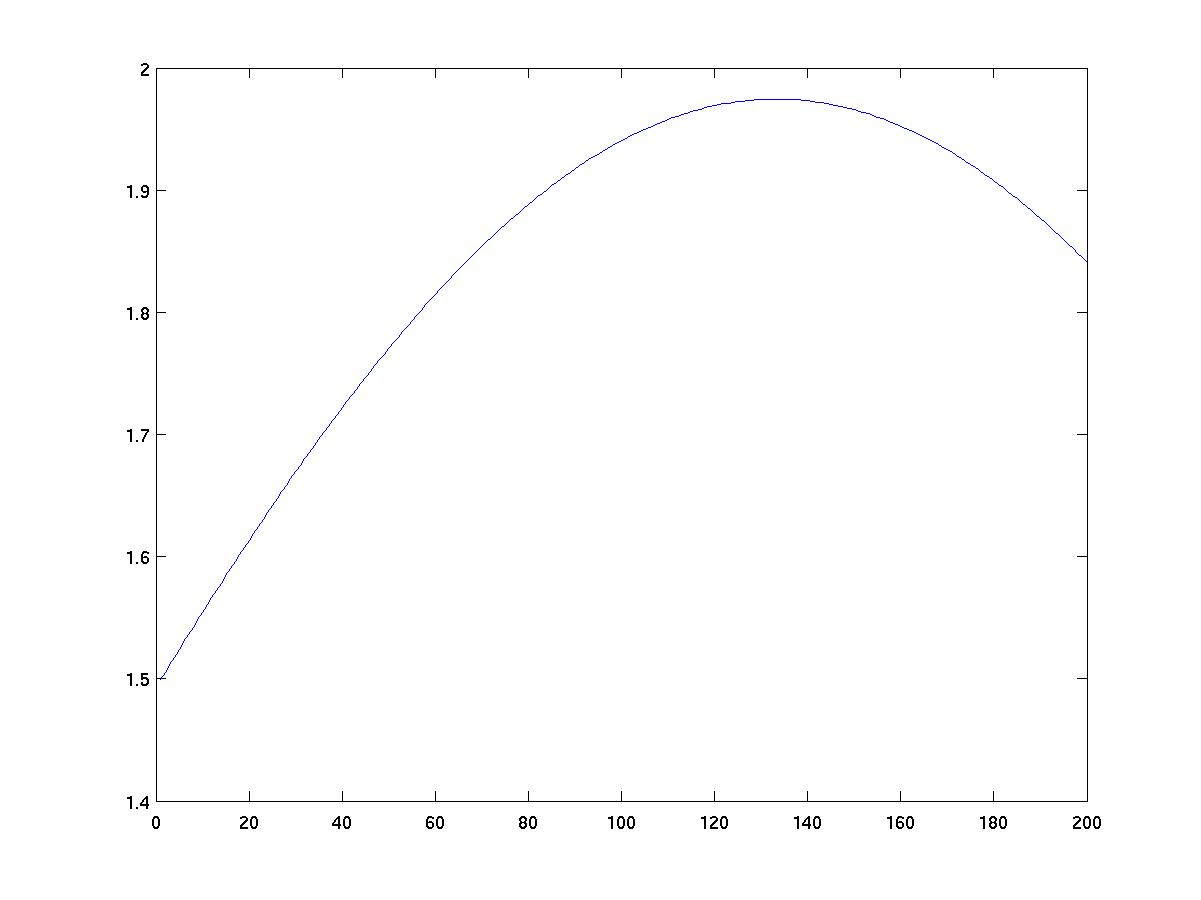
width=2

width=5

width=10

width=50
